How to Find the Rate of Change: Effective Techniques for 2025
The concept of the **rate of change** is fundamental in mathematics, particularly in calculus, where it plays a significant role in understanding how functions behave over time. In this article, we will dive into various methods to find the **rate of change**, including the **average rate of change**, **instantaneous rate of change**, and how these concepts apply to different mathematical scenarios.
Understanding the Rate of Change
The **rate of change** refers to how a quantity changes in relation to another quantity. In mathematics, especially in calculus, this is crucial when analyzing the behavior of functions. Types of rates include the **average rate of change**, which measures how much a function value changes over a specific interval, and the **instantaneous rate of change**, which gives us the slope of a tangent line at a single point. Understanding these rates enhances our ability to solve real-world problems effectively.
The Average Rate of Change Formula
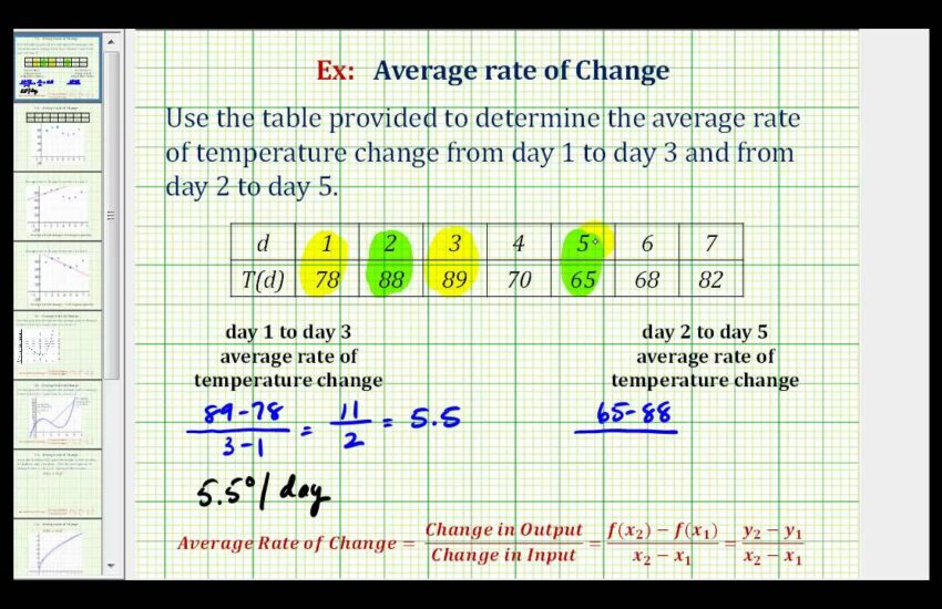
The **rate of change formula** can be defined using the **average rate of change**. To compute this, we use the formula:
Average Rate of Change = (f(b) – f(a)) / (b – a).
Here, f(a) and f(b) are the function values at points ‘a’ and ‘b’ respectively. This equation gives insight into how a function’s value changes on average between two points. For example, if a car’s position is given by a function and we wish to find the **average speed** over a specific time interval, we utilize this formula to determine how the car’s position changes over that period.
Explaining the Instantaneous Rate of Change
The **instantaneous rate of change** is defined as the limit of the average rate of change as the interval narrows down to zero. This is where we introduce the **derivative**, a concept fundamental to calculus. If we have a function f(x), the **derivative** f’(x) provides us with the slope of the tangent line at any point x on the graph of the function. This concept allows us to determine the **velocity** of an object at an exact moment in time, as opposed to just measuring changes over intervals.
Graphical Interpretation of Rate of Change
<pA graphical interpretation helps visualize the **rate of change** through functions and graphs. When we plot a function, the **slope of a line** represents its **rate of change**. A steeper slope indicates a higher rate of change, while a flatter slope shows a lower rate. For instance, on a speed versus time graph, a line with a steep slope indicates high acceleration, while a slope close to zero would represent constant speed. This graphical method aids in interpreting how functions behave over different intervals and helps in solving **rate of change problems** effectively.
Applications of Rate of Change in Real Life
The **rate of change** is not just a theoretical concept; it has practical applications in various fields, including physics, economics, and biology. Understanding how **functions and graphs** illustrate rates is vital for scientists and engineers who analyze data trends. For example, in economics, the **rate of change in economics** helps determine price elasticity or how sensitive the demand for goods is to changes in price.
Rate of Change in Physics
In physics, the concepts of **velocity** and **acceleration** are prime examples of rates of change. For instance, if a car accelerates from a stop, the speed can be expressed as the **instantaneous rate of change** of position concerning time. Using derivatives, we can determine the acceleration as the derivative of velocity. Understanding how an object moves dynamically is crucial in fields ranging from engineering to aerodynamics.
Finding Trends with Calculus
Employing calculus principles to analyze **change over time** involves using derivatives for trend analysis. In many contexts, particularly in data analysis and predictive modeling, understanding how a variable behaves and predicting future behavior relies on evaluating limits and changes in the function value. By combining derivation with statistical techniques, we can identify trends effectively, allowing businesses to forecast sales, make efficient logistical decisions, and optimize operations.
Using Derivatives for Maxima and Minima
The **derivative** also plays a vital role in optimization problems. Finding the maximum and minimum values of a function can often be done using the first and second derivatives—also known as **finding derivatives** in calculus. By locating where f’(x) = 0, we can identify critical points that may represent peaks or valleys of the function, useful in determining profit maximization in businesses, or even minimizing costs in project management.
Calculating Rates of Change: Step-by-Step Guide
Calculating the **rate of change** can initially seem complex, but breaking it down into manageable steps can simplify the process. Below is a structured guide to help individuals calculate this effectively.
Step 1: Identify the Function
To begin with, determine the function whose rate of change you want to analyze, such as f(x) = x² + 3x – 5. It is crucial to have the function clearly defined as this will guide your calculations for calculating **change in function value**.
Step 2: Choose Your Interval
Decide the interval over which you want to check the **rate of change**. For the aforementioned function, you might choose x = 1 and x = 3. Using these two points, you will later apply them in the average rate of change formula.
Step 3: Apply the Rate of Change Formula
Now that you have the defined function and interval, substitute the values into the average rate of change formula:
(f(3) – f(1)) / (3 – 1).
Calculate f(3) and f(1) to find the change in function value and subsequently evaluate your average rate of change over the interval.
Key Takeaways
- The **average rate of change** measures how a function changes over a specific interval.
- The **instantaneous rate of change** is represented through the **derivative**, which shows the slope at a given point.
- Applications of **rate of change** can be found across various disciplines, including physics and economics.
- Calculus techniques, such as evaluating limits, are essential for calculating rates effectively.
- Graphical analysis provides a substantial aid in understanding how functions behave based on **rate of change**.
FAQ
1. What is the difference between average and instantaneous rate of change?
The **average rate of change** refers to the overall change in a function over a specific interval, while the **instantaneous rate of change** indicates the change at a precise point, determined using the **derivative**. This distinction is crucial when analyzing trends across different scopes of time.
2. How is the **slope of a line** related to the rate of change?
The **slope of a line** represents the **rate of change** between two points on a function’s graph. A steeper slope signifies a greater rate of change, revealing how quickly function values vary concerning changes in the input variable.
3. Can you provide an example of calculating average rate of change?
Certainly! For a function f(x) = x², if we calculate the **average rate of change** from x = 1 to x = 4, we follow by computing f(4) and f(1), applying the average rate of change formula:
((16 – 1) / (4 – 1)) = 5. This indicates that, on average, f(x) increases by 5 units for every one unit increase in x over this interval.
4. How do limits relate to **rates in calculus**?
Limits are foundational in calculus because they allow us to compute the **instantaneous rate of change** by examining how f(x) varies as the interval approaches zero. By applying limits in the context of previous functions, we are able to derive equational relationships vital in understanding function behavior.
5. What are practical applications of understanding rate of change?
Understanding the **rate of change** enables professionals to apply predictive modeling in various fields, such as forecasting revenue in businesses or simulating vehicular motion in engineering. This knowledge is applied in functionality assessments, logistical planning, and time management strategies.
6. What role do derivatives play in finding **maxima and minima**?
Derivatives assist in identifying maximum and minimum values of a function by helping to locate critical points where f’(x) = 0. Evaluating second derivatives offers insight into whether these points correspond to maxima or minima, aiding in optimization problems tremendously.
7. How can graphical methods help in understanding the **rate of change**?
Graphical analysis allows for visual interpreting of how functions behave with changes. By plotting functions, one can easily identify trends, slopes, and rates of change, giving powerful insights into both mathematical functions and their real-world implications.